Advanced user constraints
The present tutorial is about an advanced use of the user constraints. The difference with the basic “Modelling Features” tutorial is the non-null quadratic term, i.e. \(\left(\dot{J}\dot{q}(q, \dot{q})\right)_{usr}\neq0\).
As a reminder, user constraints are defined as follows:
The user constraint is expressed in the form: \(h_{usr}(q) = 0\)
The user has to provide, for a given configuration:
The value of the constraint: \(h_{usr}(q)\)
The Jacobian matrix of the constrain: \(J_{usr}(q)\)
The quadratic term: \(\left(\dot{J}\dot{q}(q, \dot{q})\right)_{usr}\)
The user constraints are implemented using the user_cons_hJ and user_cons_jdqd functions.
Rod-crank-piston example
The system to analyse is a simple rod-crank-piston system as it can be found in engines.
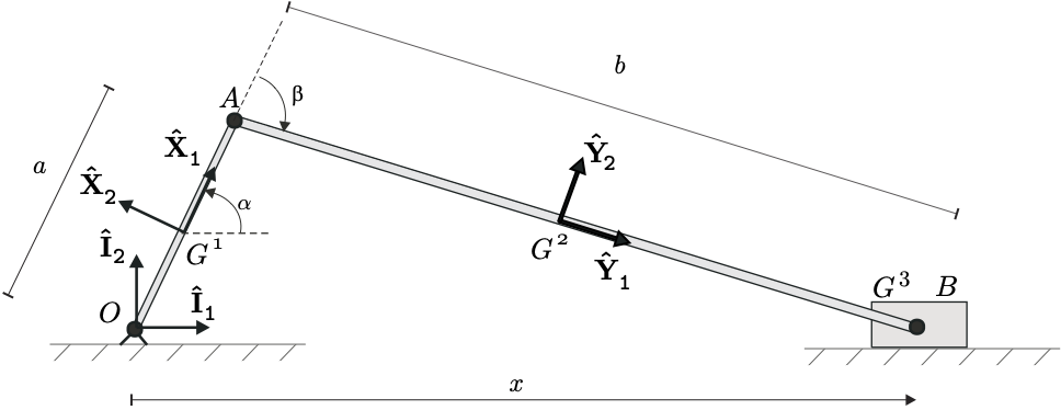
Rod-crank-piston system: definition
The model is composed of the following elements:
Three bodies
the rod \(OA\)
Length: a = 150 mm
Center of mass \(G^1\) located in the middle of the segment \(OA\)
Mass: 0.3 kg
Inertia along axis \(\hat{I}_{3}\): 0.005 kg.m2
the crank \(AB\)
Length: b = 300 mm
Center of mass \(G^2\) located in the middle of the segment \(AB\)
Mass: 0.7 kg
Inertia along axis \(\hat{I}_{3}\): 0.003 kg.m2
the piston \(B\)
Center of mass \(G^3\) located in \(B\)
Mass: 0.35 kg
Three joints
A revolute joint between the base and the rod
A revolute joint between the rod and the crank
A prismatic joint between the base and the piston
A ball cut between the crank and the piston
Forces
External torque applied on the rod in \(O\): \(T\hat{I}_{3}\) with \(T=0.5\,Nm\)
Friction force resistive to the piston motion: \(-c\dot{x}\hat{I}_{1}\) with \(c=5\,Ns/m\)
No gravity in the system
The goal is to analyze the evolution over 5sec of the system with the piston starting at the top-dead-center configuration.
Although this system has three generalized coordinates, there is only one DOF, i.e. the piston translation. Two constraints are therefore necessary to link the rotations of both rod and crank to the piston translation.
The constraints can thus be written as:
\(h_1 \triangleq a~\cos \alpha + b~\cos \left( \alpha + \beta \right) - x = 0\)
\(h_2 \triangleq a~\sin \alpha + b~\sin \left( \alpha + \beta \right) = 0\)
\(\alpha\): rod rotation;
\(\beta\): crank rotation;
\(x\): piston rotation.
The Jacobian is given by
\(J = \left( \begin{array}{rrr} - a \sin\alpha - b \sin \left( \alpha + \beta \right) & -b \sin \left( \alpha + \beta \right) & -1 \\ a \cos\alpha + b \cos \left( \alpha + \beta \right) & b \cos \left( \alpha + \beta \right) & 0 \end{array} \right)\)
Its time derivative is equal to
\(\dot{J} = \left( \begin{array}{rrr} - a \dot \alpha \cos \alpha - b (\dot \alpha + \dot \beta) \cos(\alpha + \beta) & -b (\dot \alpha + \dot \beta) \cos(\alpha + \beta) & 0 \\ - a \dot \alpha \sin \alpha - b (\dot \alpha + \dot \beta) \sin(\alpha + \beta) & -b (\dot \alpha + \dot \beta) \sin(\alpha + \beta) & 0 \\\end{array} \right)\)
And the quadratic term \(\dot{J}\dot{q}\) is therefore
\(\begin{array}{ccl} \dot{J}\dot{q} & = & \left( \begin{array}{rrr} - a \dot \alpha \cos \alpha - b (\dot \alpha + \dot \beta) \cos(\alpha + \beta) & -b (\dot \alpha + \dot \beta) \cos(\alpha + \beta) & 0 \\ - a \dot \alpha \sin \alpha - b (\dot \alpha + \dot \beta) \sin(\alpha + \beta) & -b (\dot \alpha + \dot \beta) \sin(\alpha + \beta) & 0 \\\end{array} \right) \left( \begin{array}{c} \dot{\alpha}\\ \dot{\beta}\\ \dot{x} \end{array} \right) \\ \\ &=& \left( \begin{array}{c} - a \dot{\alpha}^2 \cos \alpha - b (\dot \alpha + \dot \beta) \dot{\alpha} \cos(\alpha + \beta) - b (\dot \alpha + \dot \beta) \dot{\beta} \cos(\alpha + \beta)\\ - a \dot{\alpha}^2 \sin \alpha - b (\dot \alpha + \dot \beta) \dot{\alpha} \sin(\alpha + \beta) - b (\dot \alpha + \dot \beta) \dot{\beta} \sin(\alpha + \beta)\\ \end{array} \right) \\ \\ &=& \left( \begin{array}{c} - a \dot{\alpha}^2 \cos \alpha - b (\dot \alpha + \dot \beta)^2 \cos(\alpha + \beta)\\ - a \dot{\alpha}^2 \sin \alpha - b (\dot \alpha + \dot \beta)^2 \sin(\alpha + \beta)\\ \end{array} \right) \end{array}\)
Step 1: Draw your multibody system
Draw the rod-crank-piston system in MBsysPad. Naming the joints is strongly recommended. Set both rod and crank rotations as dependent.
There is no specific action to do in MBsysPad for the user constraint.
Step 2: Generate your multibody equations
You have to generate the equations of motion of the system.
Step 3: Write your user function
First, edit the user_JointForces function to add the external torque and the friction force to the system. A reminder about editing this function is available in the basic tutorial.
Edit the user_cons_hJ function:
Enter the expression of the constraint: \(h_{usr}(q)\)
Fill the jacobian matrix: \(J_{usr}(q)\)
function [h,Jac] = user_cons_hJ(mbs_data,tsim)
   %...

   % retrieve joints ID
   [idR3_rod, idR3_crank, idT1_piston] = mbs_get_joint_id(MBS_info, 'R3_rod', 'R3_crank', 'T1_piston');

   % define current variables
   a_length = 0.15;
   b_length = 0.3;
   alpha = mbs_data.q(idR3_rod);
   beta = mbs_data.q(idR3_crank);
   x = mbs_data.q(idT1_piston);

   % define the value of the constraints
   h(1) = a_length*cos(alpha) + b_length*cos(alpha+beta) - x;
   h(2) = a_length*sin(alpha) + b_length*sin(alpha+beta);

   % define the value of the jacobian matrix
   Jac(1,idR3_rod) = -a_length*sin(alpha) - b_length*sin(alpha+beta);
   Jac(1,idR3_crank) = -b_length*sin(alpha+beta);
   Jac(1,idT1_piston) = -1

   Jac(2,idR3_rod) = a_length*cos(alpha) + b_length*sin(alpha+beta);
   Jac(2,idR3_crank) = b_length*cos(alpha+beta);

   %...
return
Edit the user_cons_jdqd function:
Fill the quadratic term: \(\left(\dot{J}\dot{q}(q, \dot{q})\right)_{usr}\)
function [Jdqd] = user_cons_jdqd(mbs_data,tsim)
   %...

   % retrieve joints ID
   [idR3_rod, idR3_crank] = mbs_get_joint_id(MBS_info, 'R3_rod', 'R3_crank');

   % define current variables
   a_length = 0.15;
   b_length = 0.3;
   alpha = mbs_data.q(idR3_rod);
   beta = mbs_data.q(idR3_crank);
   alpha_dot = mbs_data.qd(idR3_rod);
   beta_dot = mbs_data.qd(idR3_crank);

   % define the value of the quadratic term
   Jdqd(1) = -a_length*alpha_dot^2*cos(alpha) - b_length*(alpha_dot+beta_dot)^2*cos(alpha+beta);
   Jdqd(2) = -a_length*alpha_dot^2*sin(alpha) - b_length*(alpha_dot+beta_dot)^2*sin(alpha+beta);

   %...
return
Step 4: Run your simulation
Before running the simulation, you must modify the main script in order to indicate that there is a user constraint.
Open the exe_template.m file and add “mbs_data.Nuserc = 2;” after the project loading and before the coordinate partitioning.
The script must also call the coordinate partitioning before running the simulation. If it is not already there, add the instructions to call the coordinate partitioning module:
Open the exe_template.m file and add the following command
After the project loading (mbs_load function)
Before the time integration (mbs_exe_didryn function)
%...

MBS_user.process = 'part';

opt.part = {'rowperm','yes','threshold',1e-9,'verbose','yes'};
% Options for the coordinate partitioning.

[mbs_part,mbs_data] = mbs_exe_part(mbs_data,opt.part);
% Run the coordinate partitioning process

%...
REMARK:
More details about the options are available in the documentation.
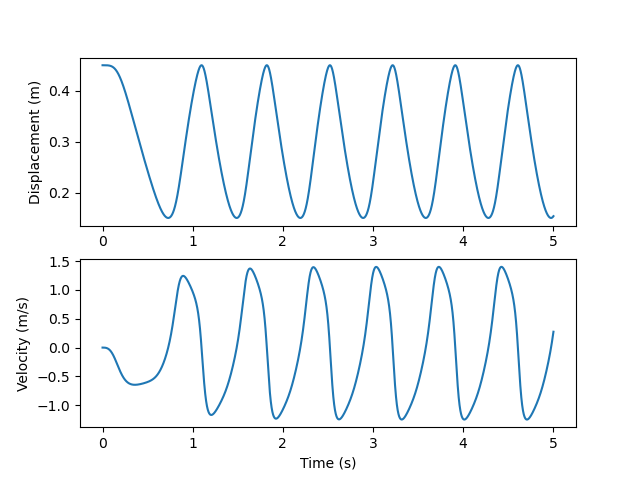
Check the results
Plot the graph of the displacement and the velocity of the piston and
check your results with the following graph.