Bodies and joints
Bodies and joints define the tree structure of the multibody systems
Bodies
They are fully defined by:
The mass
The position of center of mass
The inertia matrix
Particular points of a body can be identified using anchor points
Each body must be connected to one and only one parent joint
Joints
A joint defines the relative motion between two bodies
A joint can be attached to
The base
An anchor point
Another joint
Example: the pendulum-spring-mass system
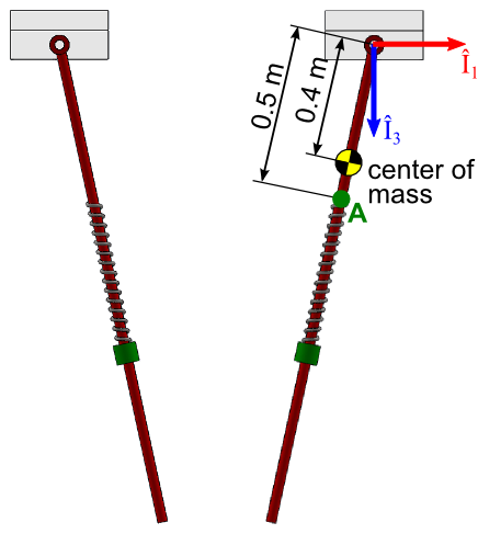
Pendulum spring illustration
REMARK:
In Robotran right handed coordinates convention is used. In this case, on the figure, positive rotations are anticlockwise
Model data
The example model is composed of the following elements:
Two bodies
the pendulum
Mass: 5 kg
Inertia along axis \(\hat{I}_{2}\): 0.1 kg.m2
the slider
Mass: 2 kg
Two joints
A revolute joint between the pendulum and the base
A prismatic joint between the pendulum and the slider
A linear spring-damper element
Will be implemented as a joint force
Stiffness: 100 N/m
Damping: 2 Ns/m
Free length: 0.1 m
Geometrical data is given in the figure above.
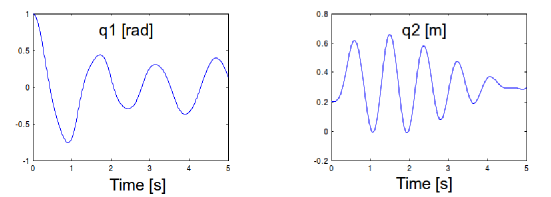
The following initial conditions are considered:
Rotation of the pendulum: 1 rad
Translation of the slider with respect to point A: 0.2 m
Step 1: Draw your multibody system
Draw a base body:
Click the body button
Select a shape
Click in the drawing area (for a rectangle: click twice: once for 1st corner and once for 2nd corner)
In the right panel, set the z component of the gravity to 9.81m/s2
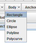
Body drop down menu
REMARK:
The shape of bodies in the 2D diagram does not influence the dynamics
Draw a R2 joint:
Click the joint button
Select R2
Click in the drawing area to draw the joint
Activate the joint properties panel by clicking on the joint
Give a name to the joint, for instance “R2_pendulum”
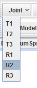
Joint drop down menu
REMARK:
In the R2 naming:
“R” stands for revolute
“2” stands for axis 2 (y-axis)
WARNING:
be careful when giving name to the elements: use only alphanumeric characters, always start with a letter (as for any variable in a program code).
Draw the pendulum body:
Same procedure as for the base body
Attach this body to the R2 joint
Activate the body properties panel by clicking on the body
In the right panel, give a name to the body and fill the dynamic properties
Center of Mass coordinates in the body-fixed frame, it is aligned with the local Z axis
Inertia matrix in the body-fixed frame, with respect to the center of mass
Pendulum body snapshot
REMARK:
When drawing a body, you can select the joint it will be attached to by coming close to this joint (which will be highlighted).
REMARK:
For each body, there is a body-fixed frame: this frame move with the body and is fixed at the position of the parent joint. Its axis are aligned with the axis of the parent body when joint positions between the 2 bodies are set to 0.
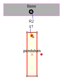
Draw an anchor point on the pendulum body:
Click the Anchor Point button
Click in the drawing area on the pendulum body
Fill the point coordinates in the right panel (coordinates in the body fixed frame, it is aligned with the local Z axis)
This anchor will be reference point for the prismatic joint.
Anchor point snapshot
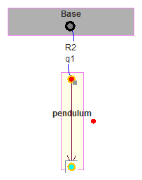
Complete the diagram:
Draw a T3 joint attached to the anchor point using the same procedure as for the R2 joint
Draw a body for the slider (Don’t forget to fill in its dynamical properties)
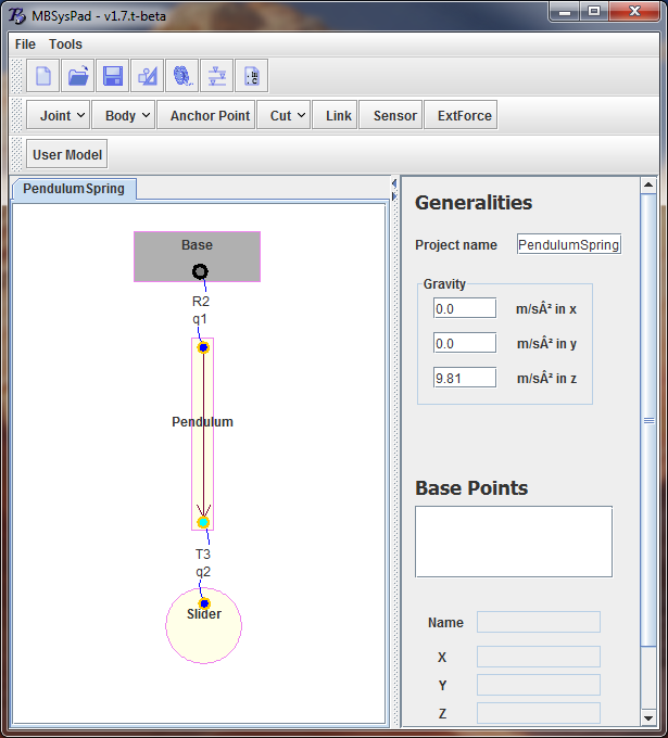
Snapshot of the complete diagram
REMARK:
In the T3 naming:
“T” stands for translation
“3” stands for axis 3 (z-axis) of the pendulum fixed-frame
Set initial conditions for the joints:
Click on the joint you want to edit
Enter the initial value at the bottom of the right panel
Save your project
REMARK:
All the data entered in MBsysPad are saved in a *.mbs file which is located in the dataR subfolder of your project. The *.mbs file uses an XML format.
Step 2: Generate your multibody equations
Click on the menu Tools > Generate Symbolic Files
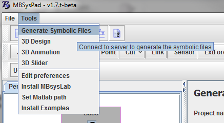
Snapshot of the Generate symbolic file menu
Enter your username and password
Select your programming language: Matlab
The language is case-sensitive;
Several language can be generated, split them with a coma;
The language of the template has te be included;
Keep other options to default
Click on the Generate button
Check that symbolic files have been downloaded to the symbolicR subfolder of your project
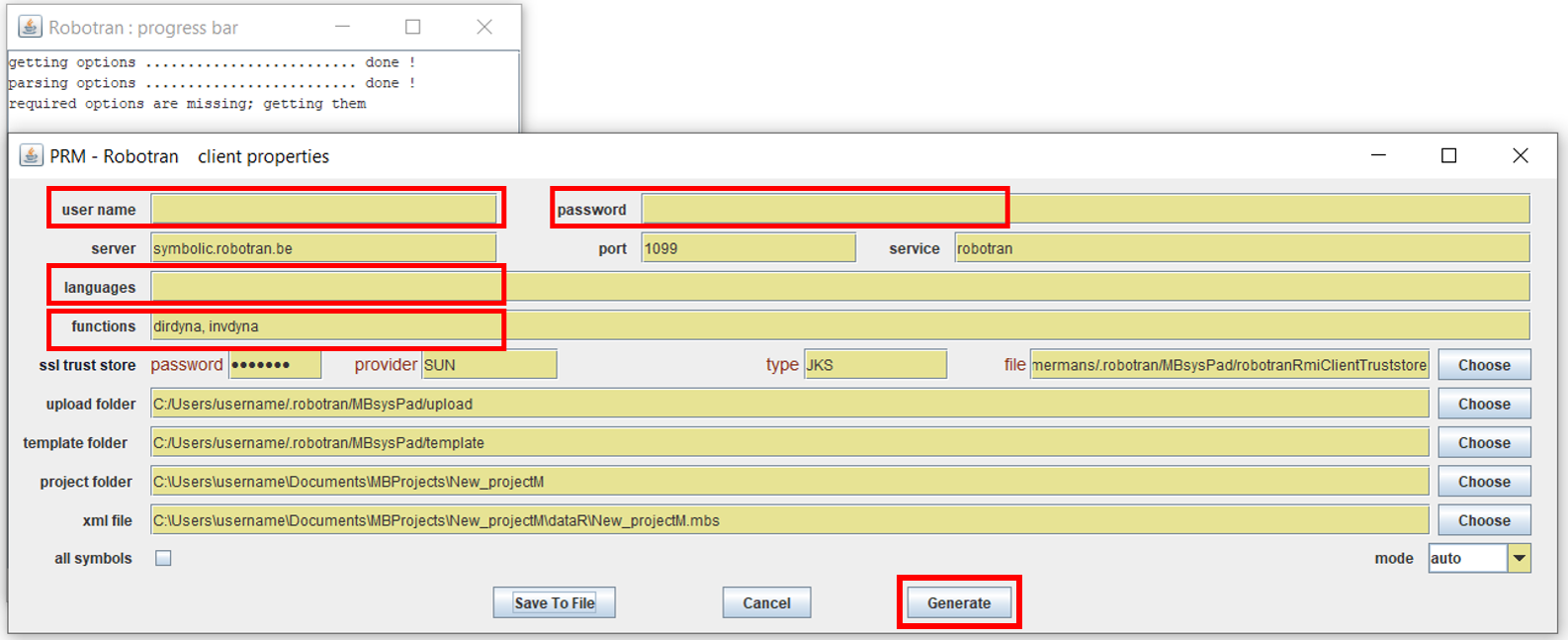
Snapshot of the symbolic generation gui
REMARKS:
If you don’t have an account you can either use demo account (usr = demo, pw = demo) or ask one via the online form Need an account ? on the Robotran website
You can save you configuration (username, password, language …) by clicking on the “Save To File” button
You can reset your parameters by clicking on “Settings->Reset password for symbolics”
Step 3: Write your user function
Open Matlab
Check that the message “MBSpath added to Matlab path” has been printed in the command window. If it was not printed:
Open MBsyspad, go to the menu: Tools > set Matlab path
Enter the path to the current directory folder of Matlab (it should be something like
C:\Users\yourusername\Documents\MATLAB)Restart Matlab
Implement the spring-damper law
Edit the user_JointForces function (located in the user_JointForces.m file from the userfctR subfolder of your project)
Write the force equations with a stifness K of 100 [N/m] and a damping C of 2 [Ns/m]
function [Qq] = user_JointForces(mbs_data, tsim)
   %...

   % set the joint force in joint 2
   id = 2;
   K = 100;
   C = 2;
   L0 = 0.1;
   Qq(id) = - ( K*(mbs_data.q(id)-L0) + C*mbs_data.qd(id) );

   %...
   return
NB :
mbs_data.q is the joint position
mbs_data.qd is the joint speed
REMARK:
A joint force/torque is a force/torque acting along the axis of a joint. It is thus:
a force for a prismatic joint,
a torque for revolute joint.
Joint forces correspond to the Qq vector in the equations of motion:
\(\begin{matrix} M(q)\ddot{q} + c(q, \dot{q}, frc, trq, g) = Q(q, \dot{q}) + J^T\lambda \\ h(q) = 0 \end{matrix}\)
Qq is the force/torque acting from the parent body to the child body. The reaction is automatically taken into account by the multibody formalism.
Step 4: Run your simulation
Set the Matlab current directory to the workR subfolder of your project
Open the exe_template.m file located in your workR folder
Check that the name of the project at the line
prjname = ...is the same as your .mbs fileMBsyspad should have create the file with your project name already included.
You have to update the name if you retrieve the file from an older project.
Run the file (either all at once or step by step using the cell mode)
REMARK:
The project data is loaded from the *.mbs using the mbs_load function. This function returns 2 structures:
mbs_data: contains variables and parameters used for the simulation
mbs_info: contains more details info such as the name of the joints, bodies, …
REMARK:
The simulation is launched using the mbs_exe_dirdyn function. This function returns the mbs_dirdyn structure which contains the time history of various quantities.
Step 5: Animate your 3D MBS
Draw your MBS system in 3D
You can customize the 3D view of your system as follows:
Open your *.mbs file in MBsysPad
Click on the Design 3D model button
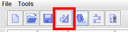
Snapshot of the Design 3D icon
Activate the body you want to edit
Click on the body in the 2D view
Or go to the 3D view and, in the right panel, use the drop down menu of the Comp tab
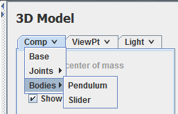
Snapshot of the 3D object selection menu
Add a shape and edit its properties
The shape inline allow to add a 3D part exported from CAD software. The part must be saved in the VRML format (extension *.wrl). Only VRML 2.0 or VRML 97 are supported (not VRML 1.0).
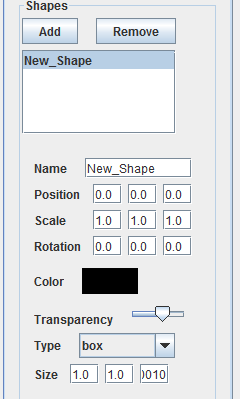
Snapshot of the 3D properties panel for bodies
Use the ViewPt to add registered viewpoint
Use the Light tab to add lights to the scene
REMARK:
Attaching a viewpoint or a light to a joint will make them follow the motion when animating the model.
Animate your results
You can view a 3D animation of the system using MBSysPad as follows:
Open your *.mbs file in MBsysPad
Click on the Animate 3D model button
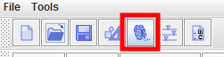
Snapshot of the Animate 3D icon
Load the result file
Click on the Open button
Select the *.anim file located in the animationR subfolder of your project

Snapshot of the Open file button
Use the control buttons to run the animation
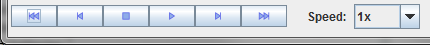
Snapshot of the Control toolbar of the Animate 3D frame
REMARK:
Navigating in the 3D view:
Rotation : Mouse motion + left button
Zoom : Mouse motion + middle button (OR ALT + mouse motion + single button)
Translation : Mouse motion + right button