Equilibrium
Introduction
This tutorial introduces the equilibrium module in Robotran. You should already be comfortable with the basics modelling features of the Getting started tutorial of Robotran.
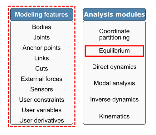
Features summary
For the moment, the tutorial for Matlab language is not available. However the theoretical aspects described below in C are still applicable for any language.
Equilibrium principle
In the case of a closed-loop multibody system, the equilibrium is computed based on the reduced equations of motions (see Robotran Basics). Generalized accelerations \(\ddot{\mathbf{q}}_\mathbf{u}\) are set to zero, the remaining reduced force term is then a set of non-linear equations which can be solved numerically to obtain the equilibrium configuration:
\(\mathbf{F_r}(\mathbf{q_u}, \dot{\mathbf{q}}_\mathbf{u}) = \mathbf{0}\)
This system of equations can be solved with the help of a Newton-Raphson method. If \(\mathbf{F}\) denotes the equations to cancel, the Newton-Raphson algorithm iterates on the equilibrium variables \(\mathbf{x}\) until the equilibrium state is obtained.
\(\mathbf{x}_{k+1} = \mathbf{x}_{k} - \left(\dfrac{\partial \mathbf{F} }{ \partial \mathbf{x} } \left( \mathbf{x}_{k} \right)\right)^{-1} \mathbf{F}\left( \mathbf{x}_{k} \right)\)
The equilibrium can either be static or quasistatic depending on the equilibrium variables considered. During an equilibrium process variables can be ignored, exchanged or added.
Example - the cart pendulum with spring
For this tutorial, let us consider the pendulum from the “modelling features” tutorial. The complex pendulum (with its four bar mechanism and its spring) is mounted on a cart. The cart slides horizontally on the ground and the pendulum rotates with respect to the cart.
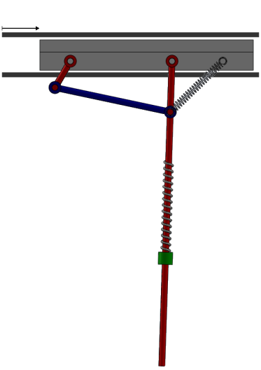
Illustration of the modified example with the four-bar pendulum mounted on a cart
The system contains a kinematic loop implying independent and dependent variables. There are three 3 independent variables: \(\mathbf{q_u} = \left[ q_1,q_2,q_3 \right]\) and 2 dependent variables: \(\mathbf{q_v} = \left[ q_4,q_5 \right]\)
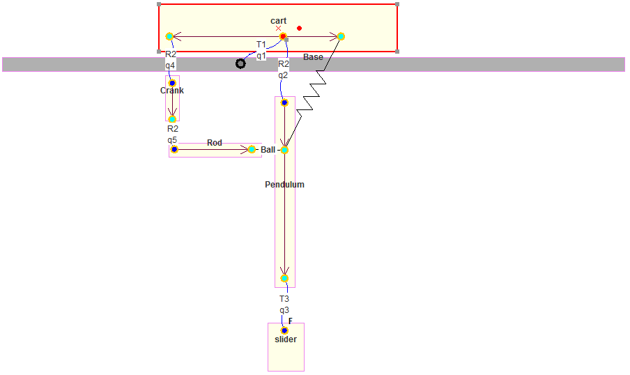
MBSysPad diagram of the four-bar pendulum mounted on a cart
REMARK:
Do not forget to implement the constitutive law (spring-damper) for the joint force (between the pendulum and the slider) but also for the spring force (between the cart and the pendulum).
It is possible to reuse your previous model (from the “modelling features”) by adding the cart and its translation d.o.f. (see section “MBsysPad 2D diagram manipulation” in “Tips and tricks”)
Static Equilibrium
For static equilibrium, the generalized velocities \(\dot{\mathbf{q}}_{\mathbf{u}}\) are set to zero. In that case, the equilibrium variables are the 3 independent coordinates, \(\mathbf{x} = \mathbf{q_u}\) and the equilibrium equations are the set of reduced equations, \(\mathbf{F} = \mathbf{F}_\mathbf{r} = \mathbf{0}\) .
REMARK:
By default, an equilibrium will be static with the free coordinates as equilibrium variables.
Non-sensitive variables
An equilibrium variable \(x_i\) can be non-sensitive with respect to the equilibrium equations \(\mathbf{F}\). This means that the variable \(x_i\) does not influence the equilibrium equations, hence its gradients is:
\(\dfrac{\partial \mathbf{F} }{ \partial x_i } = \mathbf{0}\)
The variable \(x_i\) can be ignored in the equilibrium iteration process. Its value can then be chosen arbitrarily by the user before the equilibrium process and will not evolve.
Often the non-sensitive variables are absolute positions and/or orientations. For example, the positions and orientation of a car in the horizontal plane are non-sensitive and can be chosen arbitrary.
Example - the cart pendulum with spring
Among the 3 free variables of the multibody system, the translation of the cart \(q_1\) is non-sensitive: none of the equations \(\mathbf{F_r}=\mathbf{0}\) are influenced by the cart position . Its value does not depend on the equilibrium process and can then be chosen arbitrary. However, the equilibrium state for the two remaining variables \(q_2\),\(q_3\) has to be determined.
Exchange of equilibrium variables
It is possible to replace some of the variables while performing an equilibrium. One of the free coordinates \(q_i\) can be replaced by another quantity of the system denoted by \(x_{sub}\) (e.g. a mass, a stiffness, a length, …). The equilibrium equations remain the reduced force term equalling zero, \(\mathbf{F_r} = \mathbf{0}\). In that case, the replaced free coordinates \(q_i\) are kept constant during the equilibrium process. It is important that the exchange makes sense and that the exchange variable (i.e. the new one) is sensitive to the equilibrium equations.
\(\mathbf{x} = \left[ \mathbf{q_u}\setminus \{ q_i \} , x_{sub} \right]\)
\(\mathbf{F} = \mathbf{F_r} = \mathbf{0}\) such that the pendulum is vertical
Remarks:
The exchange is not limited to one variable but can be applied to several variables at the same time
Example - the cart pendulum with spring
If we come back to the cart pendulum model, different variable exchanges can be performed. Here are some examples:
The elongation of the lower spring \(q_3\) can be set to a desired length and replaced by the spring stiffness \(k\) or its free length \(z_0\).
The pendulum angular position can be set and replaced by
the upper spring stiffness \(K\) or its free length \(Z_0\)
the joint torque applied along the pendulum \(Q_2\) or the crank rotational axis \(Q_4\).
The crank angular position can be set and replaced by
the length of the rod
the distance between the pendulum the crank attachment point with the cart.
Remarks:
The exchange and the desired equilibrium configuration has to make sense otherwise the equilibrium results could be inconsistent from a physical point of view (negative mass or negative free length for a spring)
In this tutorial, The exchange consists of setting the angular position of the pendulum to 0 radian and replacing it by the upper spring free length. The algorithm will then determine the free length and the other variables values (i.e. cart position \(q_1\) and the lower spring elongation \(q_3\)) such that the pendulum is vertical.
There you can see the printout of the equilibrium results. The cart position is again detected as non-sensitive and is kept to its zero initial value. The pendulum is angled at 0 radian (print mbs_data to verify) and the free length of the upper spring \(x_{2}\) is found to be much longer it was than initially (the spring is now working in compression while working in extension initially). The slider elongation is slightly larger than initially.
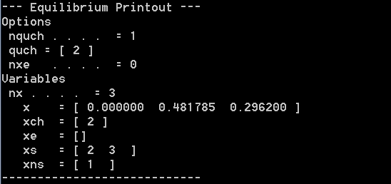
Printout for an equilibrium with exchange
Extra Equilibrium variables
Another feature of the equilibrium module is the addition of equilibrium variables and equations. One equation of equilibrium \(F_{e} = 0\) can be added to the initial equations \(\mathbf{F_r} = \mathbf{0}\) as far as one equilibrium variable \(x_{e}\) is also added. This added variable has to be sensitive with respect to the added equation.
\(\mathbf{x} = \left[ \mathbf{q_u} , x_{e} \right]\)
\(\mathbf{F} = \left[ \mathbf{F_r} , F_e \right] = \mathbf{0}\)
Remarks:
The addition is not limited to one equation and one variable, several pairs of those can be added at the same time.
Such features can be practical for adjustments of any kind (geometry, … ) which would imply complex relationship between the variables. For example, the front wheels alignement for a car can be adjusted by varying the steering rod length. The 2 added equations are used to express that the toe of the wheels has to be equal to a given value. The 2 added variables are the steering rods lengths.
Example - the cart pendulum with spring
If we come back to the cart pendulum example, several equation additions can be performed. Let us assume that the slider needs to be horizontally offset of 0.2 meter from the pendulum anchor point on the cart. This condition can be written as an additional equilibrium equation.
Quasistatic Equilibrium
A quasistatic equilibrium is a special type of equilibrium such that there is one joint i with a non-zero velocity \(\dot{q}_i\). Forces (or torques) \(F_{qstc}\) act against resistance forces (often friction) to maintain the vehicle in a continuous constant motion. There are two ways to compute the equilibrium:
Fix the speed and determine the forces (or torques) necessary to maintain this speed.
Fix the forces (or torques) applied on the system and determine the resulting speed.
Computing those equilibrium utilizes the notion of non-sensitive variable and exchange of variables. In quasistatic equilibrium, the position \(q_i\) associated with the non-zero speed is not relevant and can then be considered non-sensitive. This variable can be removed from the set of equilibrium variables and exchanged for a sensitive variable. Depending on which approach is chosen, the exchange variable is the force or the speed \(\dot{q}_i\)
Fixed speed
\(\dot{q}_i \rightarrow \mathbf{x} = \left[ \mathbf{q_u}\setminus \{ q_i \} , F_{qstc} \right] \phantom{.....} \mathbf{F}(\mathbf{x})=\mathbf{0}\)
Fixed force
\(F_{qstc} \rightarrow \mathbf{x} = \left[ \mathbf{q_u}\setminus \{ q_i \} , \dot{q}_i \right] \phantom{.....} \mathbf{F}(\mathbf{x})=\mathbf{0}\)
It is important to notice that the exchange only concerns the joint i and that the other free independent variables from \(\mathbf{q_u}\) are still part of the equilibrium process.
Remarks:
The quasistatic force \(F_{qstc}\) can be of different natures, it can either be a joint force or an external force.
The main application of quasistatic equilibrium is in vehicule dynamics where equilibrium can be performed in straight line and in curves. Multiple wheels does however require good understanding of the module features: for a fixed speed, both forces and speeds need to be exchanged in the process.
Example - the cart pendulum with spring
So far, the cart translation has not been subjected to any calculation as it was non-sensitive. A quasistatic equilibrium can be performed for the cart translation speed but it will make sense only if there is a resistive force (i.e. aerodynamic drag) . In this example, the quasistatic force \(F_{qstc}\) can simply be a joint force \(Q_{1}\) applied between the ground and the cart (i.e. a linear actuator).
The first step is to implement an aerodynamic drag force on the slider.
Add a Force sensor on the slider, name it and regenerate the equations with MBSysPad
Implement the aerodynamic force as a function of the slider angle \(\theta\) of attack and its horizontal velocity \(v\) :
\(F_{aero} = - a v^2 \left(b - \sin(2\theta)(b-c) \right)\)
Remarks:
Limit yourself to speed less than 10 m/s for the cart. Otherwise, equilibrium might not converge or encounter undesired solution (reverse four-bar configuration)
Qa stands for actuated torques/forces, while Qq is the joint torques/forces.