Cuts
A cut is used to deal with system containing kinematic loops: the loop is cut to recover a tree-like structure.
When inserting a cut in the system, the corresponding algebraic constraint equation and their Jacobian matrix will be generated.
Three kinds of cuts are implemented in Robotran:
The rod cut -> it imposes a constant length between two points of the system -> 1 algebraic constraint.
The ball cut -> it imposes that the two connected points are merged -> 3 algebraic constraints.
The solid cut -> it imposes that two bodies are coincident -> 6 algebraic constraints.
The rod cut
The rod cut applies to kinematic loops wich contains a connecting rod.
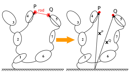
Illustration of the rod cut concept using a potato multibody diagram
The rod cut imposes one algebraic constraint: the distance between the two connecting point must remain constant and equal to a given value.
In practice, for computation efficiency, the closure condition is writtent using the square of the length:\(\begin{equation} \begin{split}h(q,t) &\triangleq \frac{1}{2} \parallel x^{PQ}(q,t)\parallel^2 - \frac{l^2}{2} \\ &= \frac{1}{2} x^{PQ}(q,t) \cdot x^{PQ}(q,t) - \frac{l^2}{2}\\ &= 0 \\ \end{split} \end{equation}\)
WARNING:
The length of the rod specified in MBsysPad can not be null.
The ball cut
The ball cut applies to kinematic loops which contains a ball joint.
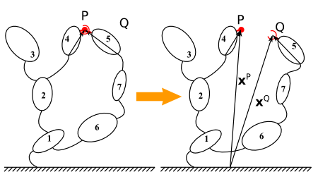
Illustration of the ball cut concept using a potato multibody diagram
The ball joint can be considered as “ideal”:
From geometrical point of view (no backlash);
From dynamic point of view (no torque transmitted).
The ball cut equivalent imposes three position constraints: the position vectors of the two connecting point must coincide at any time: \(h(q,t) \triangleq x^Q(q,t) - x^P(q,t) = 0\)
The ball cut imposes:
3 algebraic constraints for a 3D system;
2 algebraic constraints for a 2D system (the third one will be automatically removed).
REMARK:
In MBsysPad, it is possible to manually removed one algebraic in one direction.
The solid cut
The solid cut imposes that two bodies must coincide.
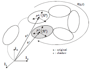
Illustration of the solid cut concept using a potato multibody diagram
The solid cut imposes 6 algebraic constraints:
3 position constraints imposing that the two bodies have a common point;
3 orientation constraints expressing that the frames of each body must coincide at any time.
Coordinate partitioning
The goal of the coordinate partitioning is to reduce the set of differential-algebraic equations to a set of ordinary differential equations.
Stating point: DAEs \(\boxed{\begin{matrix} M(q)\ddot{q} + c(q, \dot{q}, frc, trq, g) = Q(q, \dot{q}) + J^T\lambda \\ h(q) = 0 \end{matrix}}\)
The joint variables are split into 2 groups:
The independent variable u
The dependent variable v
\(\begin{equation} \boxed{q = \begin{pmatrix}u \\ v \end{pmatrix} ; J = \begin{pmatrix}J_{u} & J_{v} \end{pmatrix}} \end{equation}\)
and the differential equations can be separated accordingly
\(\begin{equation} \begin{pmatrix} M_{uu} & M_{uv} \\ M_{vu} & M_{vv} \end{pmatrix} \begin{pmatrix}\ddot{u} \\ \ddot{v} \end{pmatrix} + \begin{pmatrix} c_{u} \\ c_{v} \end{pmatrix} = \begin{pmatrix} Q_{u} \\ Q_{v} \end{pmatrix} +\begin{pmatrix}J_{u}^T \\ J_{v}^T \end{pmatrix} \lambda \end{equation}\)
The dependent variables are eliminated from the differential equation by solving the constraint equations at each time step. Solving the constraint equations imply a newton-raphson procedure.
It results in a set of ODEs in terms of the independent variables.
At the end: ODEs \(\boxed{\mathcal{M}(u)\ddot{u}+\mathcal{F}(\dot{u},u) = 0}\)
REMARK:
Refer to Robotran basics for more details.
Independent variables
Their position and velocity are fixed by the time integrator
Their acceleration results of the equation of motion
Initial values must be given by the user
Dependent variables
Their values depend on the independent (and driven) variables
Their positions, velocities and accelerations are fixed by the constraint equations -> Number of dependent variables = number of independent constraints
Example: suspension with superimposed arms
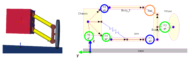
Illustration of the suspension with superimposed arms
5 generalized coordinates
2 constraints: \(\begin{matrix} x_A & = & x_B \\ y_A & = & y_B \end{matrix}\)-> 2 dependent variables to choose
\(x_A = x_B \Rightarrow l_{1}\cos(q_{2}) + l_{2}\sin(q_{2}+q_{3}) - l_{1}\cos(q_{5}) = 0\)
\(y_A = y_B \Rightarrow l_{1}\sin(q_{2}) + l_{2}\cos(q_{2}+q_{3}) - l_{1}\sin(q_{5}) - l_{2} = 0\)
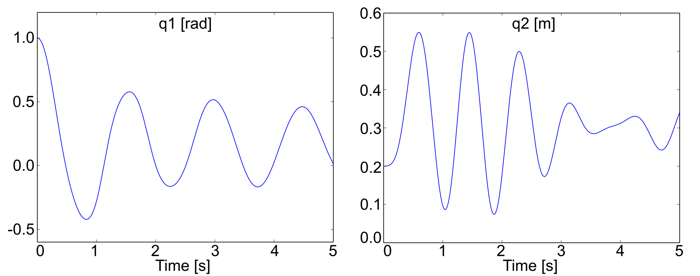
Back to the pendulum-spring example
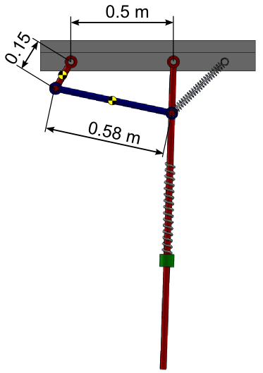
Illustration of the modified example with a kinematic loop
Add a four bar mechanism with the following additional bodies:
The crank connected to the ground
Mass: 2 kg
Inertia along axis \(\hat{I}_{2}\): 0.1 kg m²
Center of mass: in the middle of the crank
The rod connected to the crank and to the pendulum
Mass: 2 kg
Inertia along axis \(\hat{I}_{2}\): 0.1 kg m²
Center of mass: in the middle of the rod
The joint between the pendulum and the blue rod will be replaced by a ball cut.
Step 1: Draw your multibody system
Open the Pendulum Spring model in MBsysPad
Add an anchor point on the base and fill the coordinates
The anchor point on the pendulum has been created here
REMARK:
A single anchor point can be used for connecting several elements: a joint, a link, a cut …
Add the kinematic chain of the crank and the rod
Add a ball cut between the rod and the pendulum
Click on the Cut button and select ball
Click on the anchor point of the pendulum
Click on the anchor point of the rod
Click on the cut to edit its properties
Change the name of the cut
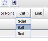
Menu to create a ball cut
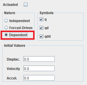
Set the joint between the base and the crank and the joint between the crank and the rod as dependent variables:
Click on the joint
Click on dependent (see figure below, on the red rectangle)
REMARK:
The initial value of the dependent joint can be arbitrary, the newton-raphson procedure will modify the value in order to close the loop. However, this procedure will choose one solution among the existing solutions. For example the loop closure can be solved with the configuration shown in the previous figure or it can put the crank upward.
To drive the newton-raphson procedure toward the solution you want, you have to adjust the initial value of the joints to be close of your loop closure solution.
Joint nature gui screenshot
REMARK:
You can set or modify the choice of dependent (and independent) variable in the code. This feature is only recommended for advanced users.
Warning: any change of joint nature done in MBsysPad will be overwrote by the code!
The ID number of the joint is valid for our project, these numbers can differ for your project. See the Tips and tricks in order to get a strong method of joint ID recovering.
Setting joint nature in the code (Optional, for advanced users)
Open the exe_template.m file and add the following command
After the project loading (mbs_load function)
Before the coordinate partitioning (mbs_exe_part function)
%...
%%%%%%%%%%%%%%%%%%%%%%%%%%%%%%%%%%%%%%%%%%%%%%%%%%%%%%%%%%%
%                 REMARK - WARNING                        %
%%%%%%%%%%%%%%%%%%%%%%%%%%%%%%%%%%%%%%%%%%%%%%%%%%%%%%%%%%%
% This code overwrites the modification done in MBsysPad. %
% For  the  next  section  of the  tutorial  you  have to %
% comment these lines or adapt the joint nature for each  %
% section.                                                %
%%%%%%%%%%%%%%%%%%%%%%%%%%%%%%%%%%%%%%%%%%%%%%%%%%%%%%%%%%%
mbs_data = mbs_set_qu(mbs_data,[1:mbs_data.Njoint])
% all variables are set to "independent"

mbs_data = mbs_set_qv(mbs_data, [3,4])
% variables 3 and 4 are set to "dependent"

%...
Step 2: Generate your multibody equations
Click on the menu Tools > Generate Symbolic Files
Follow the procedure as for the previous example
Step 3: Write your user function
No user functions are necessary when using predefined cuts
Step 4: Run your simulation
In case of kinematic loops the coordinate partitioning has to be present in the code. In most template the coordinate partitioning is present. If not you have to modify the script:
Open the exe_template.m file and add the following command
After the project loading (mbs_load function)
Before the time integration (mbs_exe_didryn function)
%...

MBS_user.process = 'part';

opt.part = {'rowperm','yes','threshold',1e-9,'verbose','yes'};
% Options for the coordinate partitioning.

[mbs_part,mbs_data] = mbs_exe_part(mbs_data,opt.part);
% Run the coordinate partitioning process

%...
REMARK:
More details about the options are available in the documentation.