Inverse dynamics
Introduction
Inverse dynamics aims at computing the joint actuation forces and torques required to satisfy a given multibody trajectory. The inverse dynamics of a multibody system is the computation of the generalized joint forces and torques applied in the joints for a given configuration or a desired trajectory of the MBS.
In case of inverse dynamics, there are many situations depending on:
The topology of the multibody system: tree-like or closed-loop.
The presence or not of driven variables.
The number of actuators with respect to the number of degrees of freedom.
The existence (possible free motion) or not (fully driven motion) of degrees of freedom in the system.
To illustrate all these situations in this tutorial, let us first visualize the following decision tree dealing with all the possibilities.
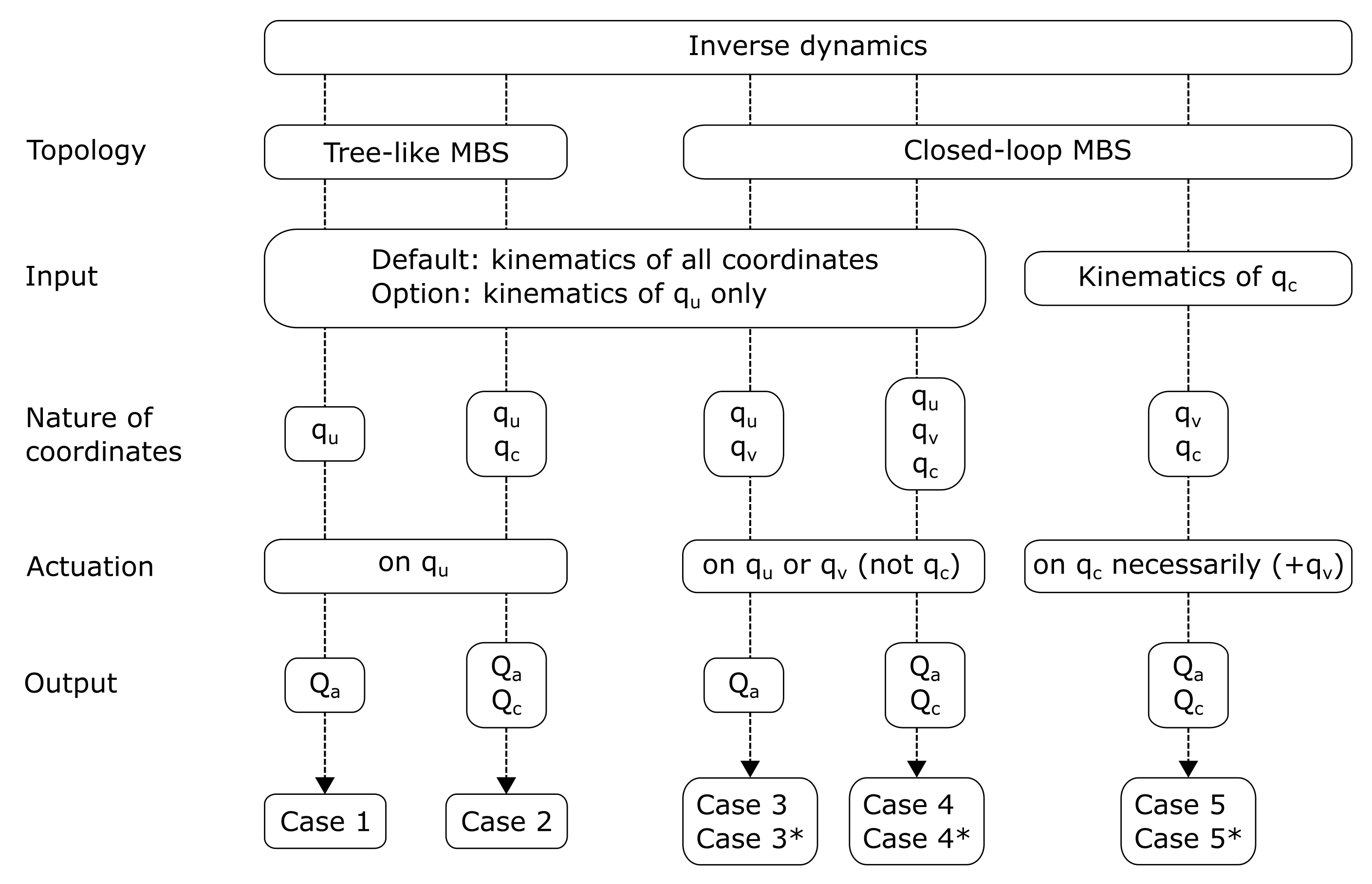
Inverse dynamics decision tree
Topology: as usual, it is very useful to distinguish the process for Tree-like and Closed-loop constraint because their modelling formalisms are quite different.
Input: two possibilities are offered to the user to introduce the MBS trajectory. Either by providing the whole set of joint coordinates or by providing only the subset of the independent coordinates (position, velocity and acceleration).
Nature of coordinates: the inverse dynamics process will be different depending on the presence or not of independent, dependent or driven variables.
Actuation: whereas for Tree-like systems actuation must always be present on all free joints (i.e. independent), for Closed-loop systems:
On the one hand, actuators can be located on independent or dependent joints.
On the other hand, the number of actuators can be equal or greater (for overactuated MBS) to the number of degrees of freedom.
Output: whereas the standard output of inverse dynamics refers to the actuation force (or torque) in the actuated joints (\(Q_a\)), the forces (and torques) in the driven joints (\(Q_c\)) being of the same nature are also useful results. ..
REMARK:
Refer to Robotran basics for more details.
Tree-like MBS
Case 1: MBS with no driven variables
Let us first define the following vector:
\(\boldsymbol{\phi}\,\triangleq\,\mathbf{M} \, \ddot{\mathbf{q}} + \mathbf{c}\)
In case of a tree-like multibody system in which all the variables are free, they can be considered as independent coordinates, i.e. \(\mathbf{q} = \mathbf{q_u}\).
In the particular case of inverse dynamics, it is necessary to distinguish the active and the passive components within the \(i^{th}\) joint force or torque \(Q^i\):
The passive component, denoted \(Q^i_p\), refers to a force (or a torque) arising from passive mechanical devices such as springs, dampers, friction elements, etc.
The active component, denoted \(Q^i_a\), refers to the force (or the torque) to actuate the joint (via any source for actuation like an electrical motor). This is what inverse dynamics aims to compute.
Given the above explanation, the inverse dynamics reads:
\(\mathbf{Q_a} = \boldsymbol{\phi}(\mathbf{q}, \dot{\mathbf{q}}, \ddot{\mathbf{q}} - \mathbf{Q_p}(\mathbf{q}, \dot{\mathbf{q}})\)
This equation represents the inverse dynamics of an unconstrained MBS, in which all the non-driven joints are actuated. There are as many unknown \(Q_a\) as equations.
Contrary to the direct dynamics for which only the initial conditions are required to simulate the MBS, the inverse dynamics requires the description of the full trajectory. In other words, joint positions, velocities and accelerations must be provided as input for the inverse dynamics.
Practically, the user must provide these values via three input files and place them in the \resultsR project folder, denoted q_motion.res, qd_motion.res, qdd_motion.res repectively.
The first column contains the time and, from the second to the last one, they contain the values of the variables.
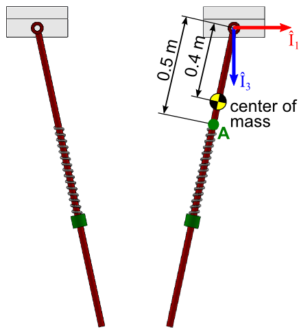
Example: the pendulum-spring-mass system
For this tutorial, let us consider the pendulum from the Bodies and joints tutorial and follow the steps 1, 2 & 3. In addition for the inverse dynamics, you must indicate which joints are actuated (step 1). For this example, variables \(\mathbf{q_1}\) & \(\mathbf{q_2}\) will be actuated in MBSysPad, as illustrated in the next figure for joint 2.
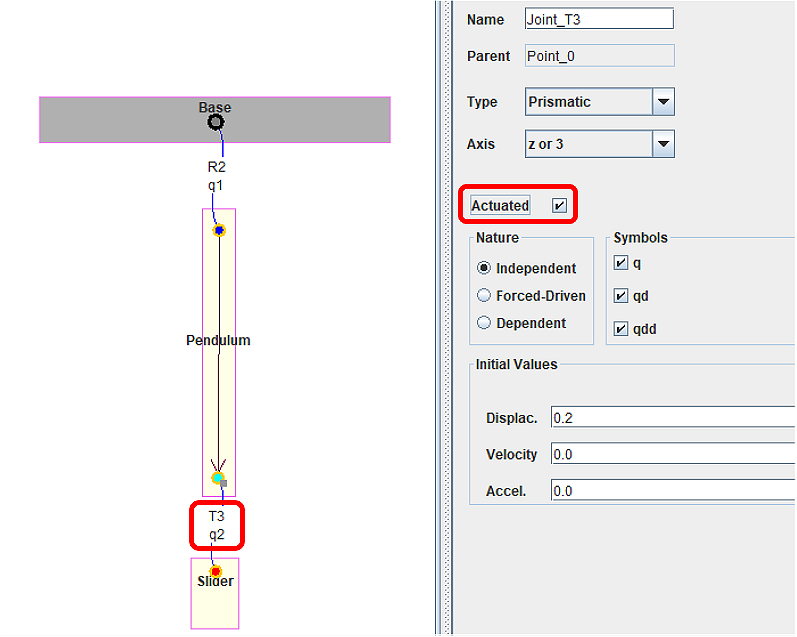
Joint 2 actuated
Pendulum spring illustration
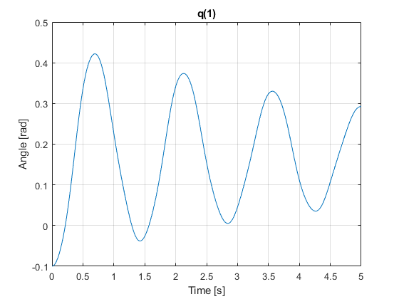
For the step 4 (Run your simulation) of the simulation as explained earlier, the trajectory of the pendulum (time history of \(\mathbf{q}, \dot{\mathbf{q}}, \ddot{\mathbf{q}}\)) is available here (input motion). Here you can see the graphs of the corresponding input motions:

The statements in your main simulation file are given here below:
%...

%==============================================================================
% Inverse Dynamics
%==============================================================================
mbs_data = mbs_set_qa(mbs_data,1);   % To set the pendulum rotation as actuated
mbs_data = mbs_set_qa(mbs_data,2);   % To set the slider translation as actuated

opt.invdyn = {'motion','trajectory',1000,'save2file','yes','renamefile','no'}; % Inverse dynamics options

[mbs_invdyn,mbs_data] = mbs_exe_invdyn(mbs_data,opt.invdyn); % Inverse dynamics process

%...
As regard the input files, they will be loaded by the user via a pop-up window appearing during the inverse dynamics simulation (first column: time, second to last column: \(Qa\)).
According to the decision tree above, the results \(Qa\) of the inverse dynamics will be stored in a file located in the \resultsR folder.
Check the results
Plot the graph of the actuation torque (joint 1) and force (joint 2).
The results are stored in the Qa field of the output structure mbs_invdyn (mbs_invdyn.Qa).
Case 2: MBS with driven variables
When the tree-like MBS contains driven variables, the inverse dynamics simulation is rather similiar to the previous one, by using the following partitioning: \(\mathbf{q} = \{\mathbf{q_u}, \mathbf{q_c}\}\), that will apply on all matrices.
For the independent joints, the inverse dynamics equations are similar to case 1 and read:
\(\mathbf{Q_a} = \boldsymbol{\phi_u}(\mathbf{q}, \dot{\mathbf{q}}, \ddot{\mathbf{q}}) - \mathbf{Q_{u,p}}(\mathbf{q_u}, \dot{\mathbf{q}}_\mathbf{u})\)
And for the driven joints, the actuation force (or torque) is computed in the \(\mathbf{Qc}\) variable corresponding to the constraint joint forces (or torques) required to satisfy the driven motion.
\(\mathbf{Q_c} = \boldsymbol{\phi_c}(\mathbf{q}, \dot{\mathbf{q}}, \ddot{\mathbf{q}}) - \mathbf{Q_{c,p}}(\mathbf{q_c}, \dot{\mathbf{q}}_\mathbf{c})\)
In this situation, the results of the inverse dynamics are of two types: \(\mathbf{Qa}\) for the actuated joints and \(\mathbf{Qc}\) for the constraint joints.
Example: the pendulum-spring-mass system
For this tutorial, let us consider the previous pendulum in which the first variable is still independent (pendulum rotation) and the second one is driven (slider translation) according to a sinusoidal motion:
\(\mathbf{q_2(t)} = \boldsymbol{0.1sin(2\pi t)}\)
Don’t forget to set \(\mathbf{q_2}\) as a driven variable and to implement the above function and its time derivatives in the user_DrivenJoint file.
Check the results
Plot the graph of the actuation torque (joint 1) and driven force (joint 2) (results are available in \resultsR folder) and check your results with the following graphs.


Constrained MBS
Case 3: MBS with no driven variables
In case of constrained MBS, the coordinate partitioning applies to the independent and dependent variables as follows: \(\mathbf{q} = \{\mathbf{q_u}, \mathbf{q_v}\}\). As for the direct dynamics, this partitioning is also applied to all the elements of the dynamic equations.
We can partition the dynamic term as follows:
\(\boldsymbol{\phi} = \{\boldsymbol{\phi_u},\boldsymbol{\phi_v}\}\)
And the generalized joint force vector as follows:
\(\boldsymbol{Q} = \{\boldsymbol{Q_u},\boldsymbol{Q_v}\}\)
The most common situation to deal with is the case where there are as many actuated joints as degrees of freedom. In short, it means that the number of \(size(Q_a) = size(Q_u)\).
Subcase 1: the actuators are located on the independent joints (\(a = u\)). The inverse dynamics model reads:
\(\mathbf{Q_a} = \mathbf{Q_{u,a}} = \boldsymbol{\phi_u} - \mathbf{Q_{u,p}} + \mathbf{B^t_{vu}}({\phi_v} - \mathbf{Q_{v,p}})\)
In which \(\mathbf{Q_{u,p}}\) and \(\mathbf{Q_{v,p}}\,\) stand for the passive joint forces (spring, damper…) in the independent and dependent joints respectively.
Subcase 2: the actuators are located either on some of the independent joints or some of the dependent joints (\(a \in \{u,v\}\)). Hence, considering a partitioning \(\mathbf{q} = \{\mathbf{q_e}, \mathbf{q_f}\}\) in which subscripts \(e\) and \(f\) refer to the active and passive joints respectively, the inverse dynamics model becomes:
\(\mathbf{Q_a} = \mathbf{Q_{e,a}} = \boldsymbol{\phi_e} - \mathbf{Q_{e,p}} + \mathbf{B^t_{ve}}({\phi_f} - \mathbf{Q_{f,p}})\)
Subcase 3 (case 3* in the Inverse dynamics decision tree): for the case of the human body and for some particular robotic applications, there are more actuated joints than degrees fo freedom. These systems refer to overactuated MBS. In such cases there is an inifinity of solutions for \(\mathbf{Q_a}\), among which one minimizes the Euclidean norm of \(\mathbf{Q_a}\). It is obtained via the pseudoinverse solution. In short, for overactuated MBS we can write the inverse dynamics model as a generic linear system of equations:
\(\mathbf{A}\,\mathbf{Q_a}=\mathbf{b}\)
In which, the rectangular \(A\) matrix possesses as many rows as degrees of freedom and as many columns as actuators (with #rows < #columns). Let us write the pseudoinverse solution as follows:
\(\mathbf{Q_a}=\mathbf{pinv(A)}\mathbf{b}\)
This is the solution given by Robotran for the inverse dynamics of overactuated systems.
Case 4: MBS with driven variables
When the tree-like MBS contains driven variables, the inverse dynamics simulation is rather similiar to the previous one, by using the following partitioning: \(\mathbf{q} = \{\mathbf{q_u}, \mathbf{q_c}\}\), that will apply on all matrices.
Let us consider the case where the actuated joints are located on the indpendent ones \((a=u)\), the inverse dynamics is similar to case 3 and reads:
\(\mathbf{Q_a} = \mathbf{Q_{u,a}} = \boldsymbol{\phi_u} - \mathbf{Q_{u,p}} + \mathbf{B^t_{vu}}({\phi_v} - \mathbf{Q_{v,p}})\)
For the driven joints, the actuation force (or torque) is computed in the \(\mathbf{Qc}\) variable corresponding to the constraint joint forces (or torques) required to satisfy the driven motion.
\(\mathbf{Q_c} = \boldsymbol{\phi_c} - \mathbf{Q_{c,p}} + \mathbf{B^t_{vc}}({\phi_v} - \mathbf{Q_{v,p}})\)
In this situation, as for tree-like systems, the results of the inverse dynamics are of two types: \(\mathbf{Qa}\) for the actuated joints and \(\mathbf{Qc}\) for the constraint joints.
As for case 3, the three subcases can be encountered, i.e.:
The actuators are on the independent joints (subcase 1).
The actuators are on independent or dependent joints (subcase 2).
The actuators are more numerous than the degrees of freedom (subcase 3, overactuation system).
Case 5: fully driven MBS
This last case is a bit particular since it relates to systems with 0 degree of freedom. In other words, they only contain dependent and driven variables and no more independent ones, giving rise to \(\mathbf{q} = \{\mathbf{c}, \mathbf{v}\}\). Here, the actuation will be located on the driven joints (\(a=c\), case 5 in the Inverse dynamics decision tree) or possibly on some of the dependent joint for overactuated system (\(a \in \{c,v\}\), case 5* in the Inverse dynamics decision tree).
Insofar as there are no more degrees of freedom, no input file is necessary for the simulation. Indeed, the motion is fully described by the driven variable time history (\(q_c=f(t)\)) provided by the user in the user driven joint function.
Example: the pendulum-spring-mass system
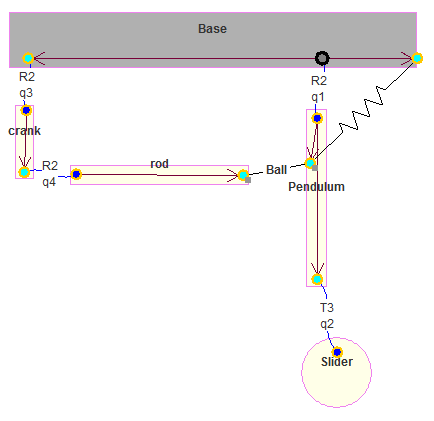
The example model is composed of the following elements:
4 bodies:
the Pendulum
the Slider
the Rod
the Crank
4 joints:
\(\mathbf{q_1}\): a revolute joint between the Pendulum and the Base.
\(\mathbf{q_2}\): a prismatic joint between the Pendulum and the Slider.
\(\mathbf{q_3}\): a revolute joint between the Crank and the Base.
\(\mathbf{q_4}\): a revolute joint between the Rod and the Crank.
Ball cut that defines the rotation of the Rod with respect to the Pendulum.
A linear spring-damper is an element that connects the pendulum and the base and it is implemented as a joint force.
The system is subject to a gravity of \(9.81\,m/s^2\).
All the input motion data for the constrained MBS is available here.
Pendulum spring, constrained MBS
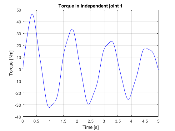
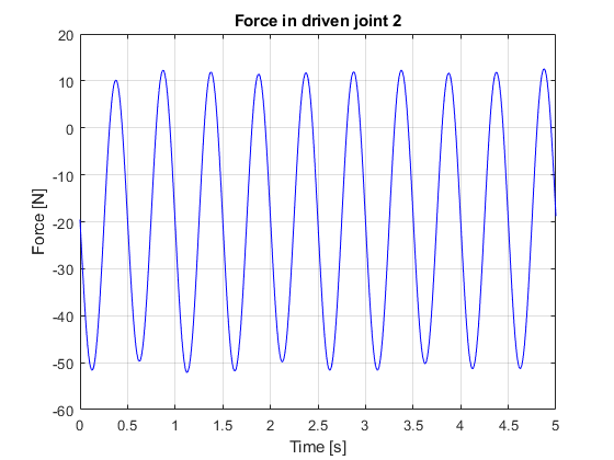
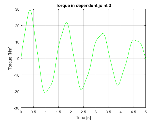
For the case 4 (subcase 1):
The joint 1 is independent.
The joint 2 is driven.
The joints 3 & 4 are dependent.
Set the joint 1 (the Pendulum rotation) as actuated.
The statements in your main simulation file are given here below:
%...

%==============================================================================
% Inverse Dynamics
%==============================================================================
mbs_data = mbs_set_qa(mbs_data,1);   % To set the pendulum rotation as actuated

opt.invdyn = {'motion','trajectory',1000,'save2file','yes','renamefile','no'}; % Inverse dynamics options

[mbs_invdyn,mbs_data] = mbs_exe_invdyn(mbs_data,opt.invdyn); % Inverse dynamics process

%...
As regard the input files, they will be loaded by the user via a pop-up window appearing during the inverse dynamics simulation (first column: time, second to last column: \(Qa\)).
Regarding the joint forces, they are defined as follows in the user_JointForces file:
function [Qq] = user_JointForces(mbs_data,tsim);

%...

if MBS_user.frott == 1
    Qq(1) = -10*mbs_data.qd(1);
    Qq(3) = -10*mbs_data.qd(3);
end

%...
Regarding the driven joints, they are defined as follows in the user_DrivenJoints file:
function [q,qd,qdd] = user_DrivenJoints(mbs_data,tsim)

%...

q(2) = 0.2 + 0.1*sin(4*pi*tsim);
qd(2) = 0.1*4*pi*cos(4*pi*tsim);
qdd(2) = -0.1*16*pi*pi*sin(4*pi*tsim);

if MBS_user.fulldriven == 1 % case fully driven
    q(1) = -0.1*sin(pi*tsim);
    qd(1) = -0.1*pi*cos(pi*tsim);
    qdd(1) = 0.1*pi*pi*sin(pi*tsim);
end

%...
For the case 4 (subcase 2):
The joint 1 is independent.
The joint 2 is driven.
The joints 3 & 4 are dependent.
Set the joint 3 (the Crank rotation) as actuated.
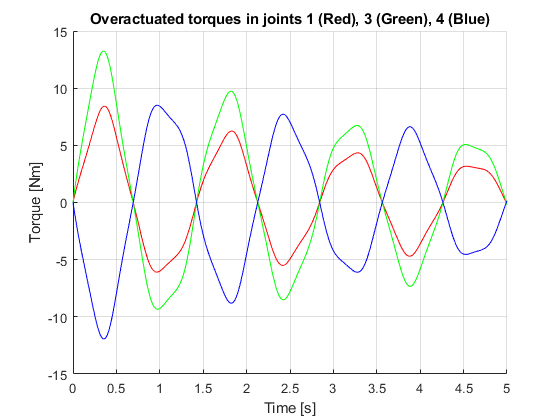
For the case 4* (subcase 3):
The joint 1 is independent.
The joint 2 is driven.
The joints 3 & 4 are dependent.
Set the joints 1, 3 & 4 as actuated.
For the case 5:
There are no independent variables.
The joints 1 & 2 are driven.
The joints 3 & 4 are dependent.
Set the joints 1 & 2 as actuated.
For the case 5*:
There are no independent variables.
The joints 1 & 2 are driven.
The joints 3 & 4 are dependent.
Set the joints 1, 2, 3 & 4 as actuated.