Modal analysis
Introduction
This tutorial introduces the modal Analysis module in Robotran. You have to be comfortable with the basics modelling features of the Getting started tutorial of Robotran.
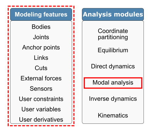
Features summary
For the moment, the tutorial for matlab language is not available. However the theoretical aspects described below in C are still applicable for any langage.
A modal Analysis is the study of the dynamic properties of systems in the frequency domain. Through the modal analysis, the eigen modes and eigen frequencies of the system are calculated. In the case of multibody system, it is particularly interesting for control purpose as it allows to identify the stable and unstable modes of the system. It is also useful to study the vibration behaviour of the system and identify critical frequencies of excitation that could lead to resonances in the system.
A modal analysis concerns the linear behaviour (small displacements) of the system around a given configuration. Therefore, it is mandatory to start from an equilibrium configuration which can be calculated with the Equilibrium module.
Modal Analysis Theory
As the linear behaviour of the system around a given configuration is of interest, the equations of motion need to be linearized around this configuration. Generally, the equations to linearize are the reduced set of equations obtained through the coordinate partitioning technique:
\(\mathbf{F_r}(\mathbf{q_u}, \dot{\mathbf{q}}_\mathbf{u}) = \mathbf{0}\)
For a general MBS model, the linearization is performed numerically, producing the following linearized system around the equilibrium configuration characterized by \(\mathbf{q}_\mathbf{u}^*\).
\(\mathbf{M_r}(\mathbf{q}_\mathbf{u}^*) \Delta \ddot{\mathbf{q}}_\mathbf{u} + \mathbf{G_r}(\mathbf{q}_\mathbf{u}^*,\dot{\mathbf{q}}_\mathbf{u}^*) \Delta \dot{\mathbf{q}}_\mathbf{u} + \mathbf{K_r}(\mathbf{q}_\mathbf{u}^*) \Delta \mathbf{q}_\mathbf{u} = \mathbf{0}\)
in which \(\Delta \mathbf{q}_\mathbf{u} = \mathbf{q}_\mathbf{u} − \mathbf{q}_\mathbf{u}^∗\), \(\mathbf{M_r}\), \(\mathbf{G_r}\),\(\mathbf{K_r}\) respectively stand for the constant mass, gyroscopic/damping and stiffness tangent matrices (size \(n−m=n_u\), the number of d.o.f.). This second-order linear system can be transformed into the following first order form:
\(\dot{\mathbf{x}}= \mathbf{A} \mathbf{x}\)
with
\(\mathbf{x}=\begin{bmatrix} \dot{\mathbf{q}}_{\mathbf{u}} \\ \mathbf{q}_{\mathbf{u}} \end{bmatrix}\rightarrow \dot{\mathbf{x}} =\begin{bmatrix} \ddot{\mathbf{q}}_{\mathbf{u}} \\ \dot{\mathbf{q}}_{\mathbf{u}} \end{bmatrix} \phantom{.....................} \mathbf{A} = \begin{bmatrix} -\mathbf{M_r}^{-1}\mathbf{G_r} & -\mathbf{M_r}^{-1}\mathbf{K_r} \\ \mathbf{I} & \mathbf{0} \end{bmatrix}\)
On this form, the eigenvalue problem can be solved determining the eigenfrequencies and the eigenmodes of the multibody system.
Modal Analysis Results
Solving the associated eigenvalue Problem, a total of \(2 n_u\)eigenvalues \(\lambda\) can be found. Each of these eigenvalues \(\lambda_i\) can be :
purely real (\(im(\lambda_i\))=0), corresponding to a non-oscillatory stable (\(\lambda_i\)<0) or non-oscillatory unstable (\(\lambda_i\)>0) eigenmode.
purely imaginary (\(re(\lambda_i\))=0),conjugate pair, corresponding to infinitively oscillating undamped eigenmode.
complex, conjugate pair, corresponding to oscillatory stable (\(re(\lambda_i\))<0) or oscillatory unstable (\(re(\lambda_i\))>0) eigenmode.
null, corresponding to a rigid mode.
A maximum of \(2 n_u\) eigenvectors \(v_i\) can be also found. Let us note that in case of multiple eigenvalues, there is only eigenvector and thus the number of eigenvectors will be less than \(2 n_u\). Moreover, in case of conjugate eigenvalues, a pair of complex conjugate eigenvectors is produced, giving rise to a single (and not two) eigenmode.
Example - the cart pendulum with spring
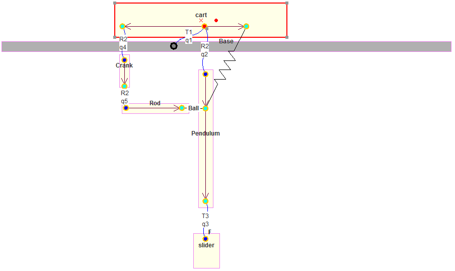
For the cart pendulum, there are three 3 independent variables: \(\mathbf{q_u} = \left[ q_1,q_2,q_3 \right]\) and 2 dependent variables: \(\mathbf{q_v} = \left[ q_4,q_5 \right]\). The linearization then results in 3 matrices of size 3 by 3.
The modal analysis (linearization, eigenvalue problem solving, post-process) are done by the modal module which is based on a structure similar to the direct dynamic module and the equilibrium module.
There you can see the printout of the modal analysis. All the different steps are correctly done.
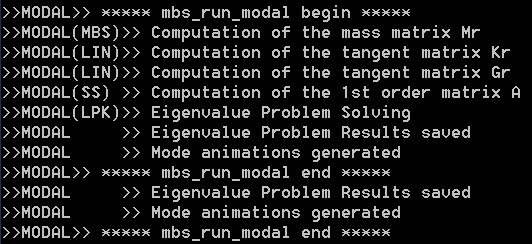
Printout for a modal analysis
A summary of the results are saved in the file modal_result.res (in the resultR folder). The first two eigenvalues are zero which correspond to one rigid mode (1 and 2). The third and forth eigenvalues are complex (conjugate pair) and correspond to a the stable oscillation of the slider on the pendulum (3 and 4). Eventually, eigenvalue 5 and 6 are also complex (conjugate pair) and correspond to the stable oscillation of both the cart and the pendulum out of phase. (Check the animationR folder and read the animated modes with MBsysPad viewer)
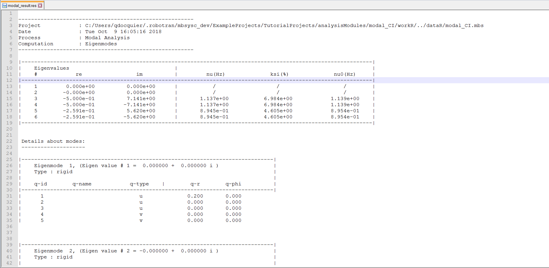
Summary of modal results
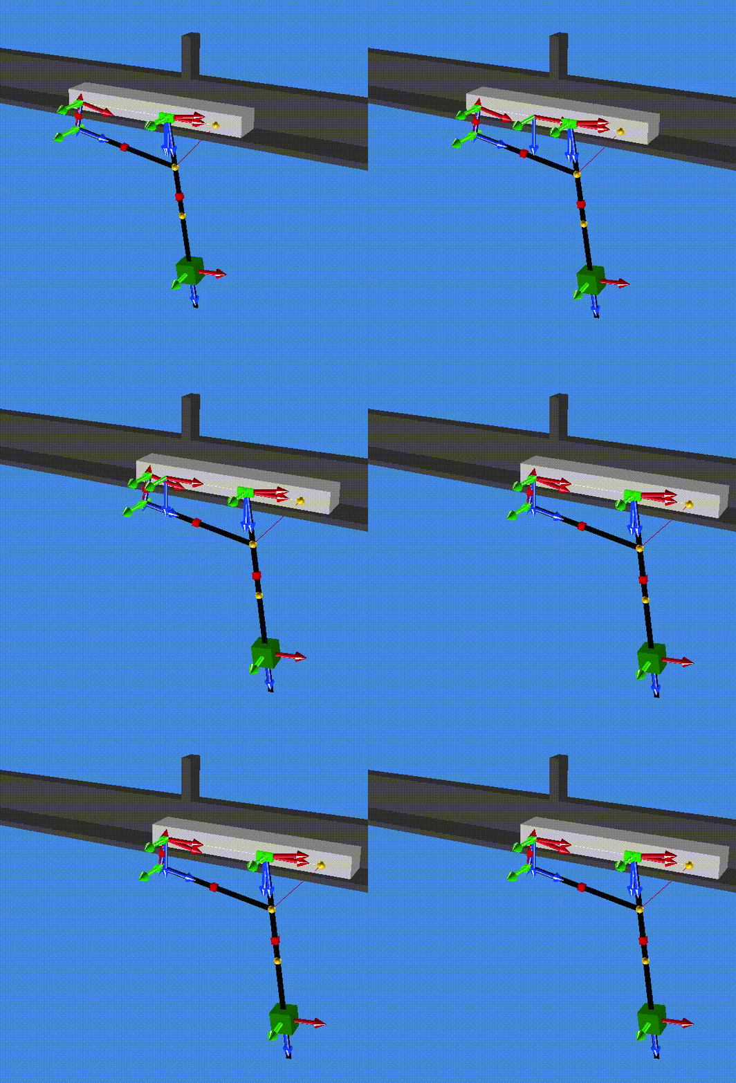
modes 1 and 2
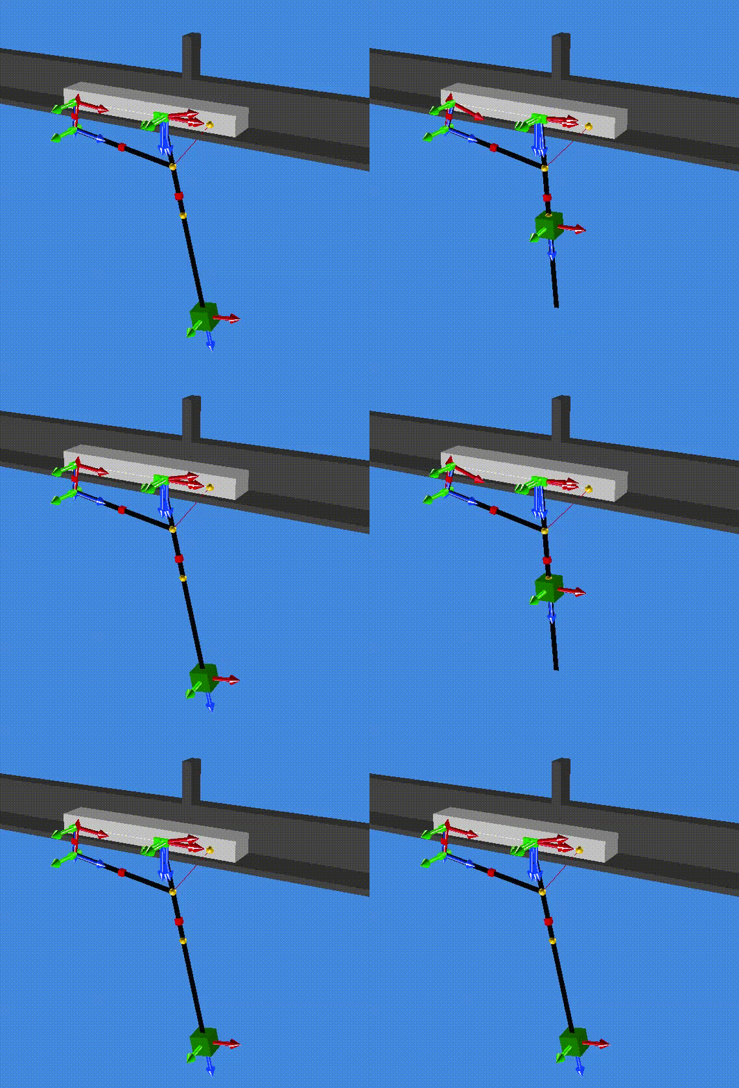
modes 3 and 4
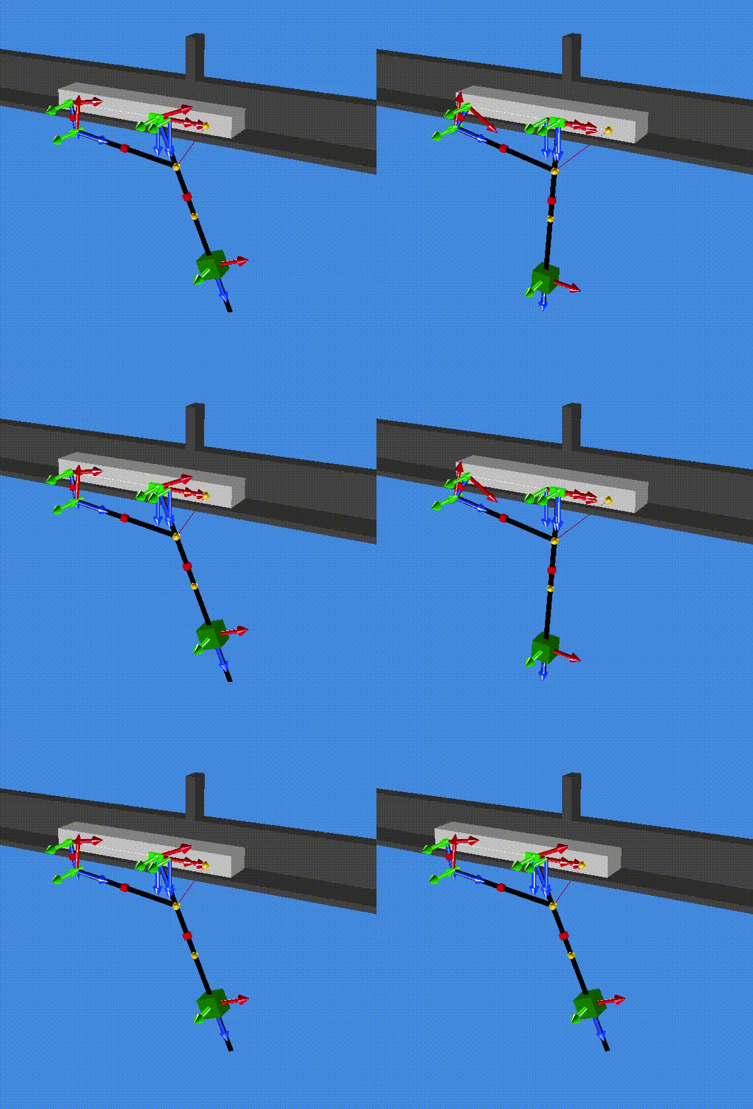
modes 5 and 6
REMARK:
In our implementation, multiple eigenmodes are produced (their animation as well).
REMARK:
It is also possible to perform a modal analysis around a quasistatic equilibrium.
