Representation of 3D forces
In the 3D window of the animation there is the option to represent the evolution of some properties of the external forces. They are two ways to represent external forces:
Visualize force components in the reference fixed-frame (the inertial frame)
Visualize force components in a moving frame
Below, there are two examples, one for each of the two above mentioned options.
REMARK: The minimum Robotran version required is v1.16.3
Basic example: visualization of force components in the reference fixed-frame
Visualizing 3D forces in MBsysPad requires additional *.anim files, one for each external force. Those files will be loaded automatically when you select the main *.anim file of your simulation (generally the main *.anim file ends by _q.anim). The steps below explain how to generate those files.
REMARK: The external force *.anim file format
The file must contain one line for each frame of the animation. The time step size between frames must be the same as in the main *.anim file. Each line must contain the following information
t_int F_I_1 F_I_2 F_I_3 M_I_1 M_I_2 M_I_3 dxF_1 dxF_2 dxF_3with:
t_int ==> the time
[F_I_1, F_I_2, F_I_3] ==> the force components in the inertial frame (as returned by the user_extForces function).
[M_I_1, M_I_2, M_I_3] ==> the torque components in the inertial frame (as returned by the user_extForces function).
[dxF_1, dxF_2, dxF_3] ==> the position of application point of the force (the point where we want to draw the force), with respect to the external force body reference point in the body fixed frame (as returned by the user_extForces function).
Step 1: Edit the user files and define the forces vector
In the user_dirdyn user file, edit the user_dirdyn_init function to initialize the forces vector:
def user_dirdyn_init(mbs_data, dd):
    #...

    # define the name and the size of the output vector
    mbs_data.define_output_vector("forces", 9)

    #...
Edit the user_ExtForces function to define the output vector. For the case of the reference fixed-frame, this vector will contain 1 value of time and 9 values that corresponds to the Swr vector: the force components in the inertial time (3), the torque components in the inertial frame (3) and the position of the application point of the force (3).
def user_ExtForces(PxF,RxF,VxF,OMxF,AxF,OMPxF,mbs_data,tsim,ixF):
    #...

    # define the vector during the direct dynamics process
    if mbs.process == 3: # the same process as that defined for the dynamics analysis

        # compute and fill the Swr vector

        # introduce the forces, torques and application point position to the output vector
        mbs_data.set_output_vector(Swr[1:],'forces')
        #the set_output_vector already automatically includes the time

    #...
Step 2: Run your simulation and obtain the forces file
Before running the simulation, you must modify the main script in order to create a file .anim that will contain the output vector defined in the previous section for each time step.
To adapt the time values to the frame rate of the animation file that you want to create, you must do an interpolation of the time and the force vector values.
Concerning the name of this file, it must follow the next structure: SimulationName_xFrc_ForceName.anim. The first part (SimulationName) must have the simulation parameter (introduced in the resfilename option), the second part is xFrc and the third one must have the name of the force in the MBsysPad model (ForceName).
Edit the main file to create the .anim file:
##==============================================================================
## Postprocess
##==============================================================================
import numpy as np
from scipy import interpolate

t_fin = mbs_dirdyn.get_options('tf') # end time
frame_rate = mbs_dirdyn.get_options('framerate') # number of frame per second for the animation file
dt = 1./frame_rate # time step
t_anim = np.arange(0, t_fin, dt) # the time values to interpolate

frc_res = np.loadtxt("../resultsR/dirdyn_forces.res") # time and force values of the simulation
frc_anim = interpolate.interp1d(frc_res[:,0], frc_res, axis=0)(t_anim) # Interpolation of forces and time
np.savetxt('../animationR/dirdyn_xFrc_LateralBumpstop.anim',frc_anim) # Save values .anim file
Step 3: Open the 3D MBS
Open your *.mbs file in MBsysPad
Click the Animate 3D Model button
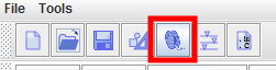
Snapshot of the Animate 3D ll icon
Load the result file
Click on the Open button
Select the .anim file equivalent to the simulation, in this casedirdyn_q.anim* (not the auxiliar .anim file created in the Postprocess)
Activate the force you want to edit
Click on the force sensor in the 2D view
Or go to the 3D view and, in the right panel, use the drop down menu of the Comp tab
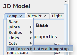
3D object selection menu
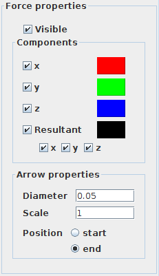
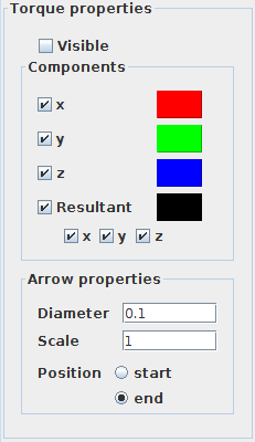
Edit the 3D force and 3D torque:
Activate or desactivate the visible components of the force/torque
Make visible the resultant of some components of the force/torque
Modifiy the arrow properties: diameter, scale and position of the arrow
Use the control buttons to run the animation and to see the force evolution
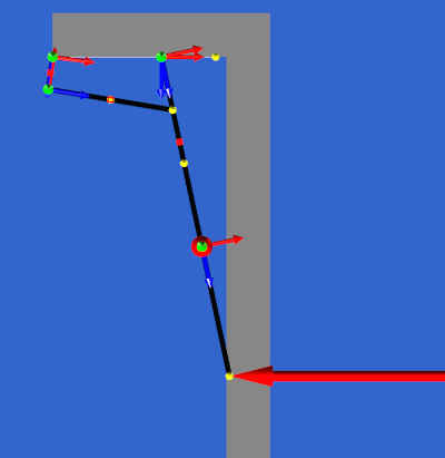
3D forces representation
REMARK:
By default, forces are displayed and torques are hidden.
REMARK:
For every force that you want to show, you will have to create a different vector, so a different .anim file. By default we allow the user to save up to 12 vectors, if you need more output value update the option
max_save_userwith the functionMbsDirdyn.set_options().
Advanced example: visualization of force components in a moving frame
Step 1: Edit the user files and define the forces vector
In the user_dirdyn user file, edit the user_dirdyn_init function to initialize the forces vector:
def user_dirdyn_init(mbs_data, dd):
    #...

    # define the name and the size of the output vector
    mbs_data.define_output_vector("forces", 15)

    #...
Edit the user_ExtForces function to define the output vector. For the case of the moving frame, this vector will contain 1 column of time, 9 columns of the Swr vector and 6 new columns that correspond to the values of the first two rows of the rotation matrix that goes from the inertial frame to the body frame (R_X_I).
import numpy as np
import MBsysPy

def user_ExtForces(PxF,RxF,VxF,OMxF,AxF,OMPxF,mbs_data,tsim,ixF):
    #...

    # define the vector during the direct dynamics process
    if mbs.process == 3: # the same process as that defined for the dynamics analysis

        # compute and fill the Swr vector

        # introduce the forces, torques, application point position and two rows of the rotation matrix to the output vector
        twoRows_R_X_I = [R_X_I_11, R_X_I_12, R_X_I_13, R_X_I_21, R_X_I_22, R_X_I_23]
        #first two rows components of the rotation matrix
        vect_forc = np.append(Swr[1:],twoRows_R_X_I)
        #adding the rotation matrix components to the vector with forces, torques & position vector
        mbs_data.set_output_vector(vect_forc,'forces')
        #the set_output_vector already automatically includes the time

    #...
REMARK: The external force *.anim file format
The file must contain one line for each frame of the animation. The time step size between frames must be the same as in the main *.anim file. Each line must contain the following information
t_int F_I_1 F_I_2 F_I_3 M_I_1 M_I_2 M_I_3 dxF_1 dxF_2 dxF_3 R_X_I_11 R_X_I_12 R_X_I_13 R_X_I_21 R_X_I_22 R_X_I_23with:
t_int ==> the time
[F_I_1, F_I_2, F_I_3] ==> the force components in the inertial frame (as returned by the user_extForces function).
[M_I_1, M_I_2, M_I_3] ==> the torque components in the inertial frame (as returned by the user_extForces function).
[dxF_1, dxF_2, dxF_3] ==> the position of application point of the force (the point where we want to draw the force), with respect to the external force body reference point in the body fixed frame (as returned by the user_extForces function).
[R_X_I_11, R_X_I_12, R_X_I_13, R_X_I_21, R_X_I_22, R_X_I_23] ==> first two rows elements of the rotation matrix that goes from the inertial frame to the frame in which the force component must be displayed. The third row is calculated internally.
Step 2: Run your simulation and obtain the forces file
Before running the simulation, you must modify the main script in order to create a file .anim that will contain the output vector defined in the previous section for each time step.
To adapt the time values to the frame rate of the animation file that you want to create, you must do an interpolation of the time and the force vector values.
Concerning the name of the file, it must follow the next structure: SimulationName_xFrc_ForceName.anim. The first part (SimulationName) must have the simulation parameter (introduced in the resfilename option), the second part is xFrc and the third one must have the name of the force in the MBsysPad model (ForceName).
Edit the main file to create the .anim file:
##==============================================================================
## Postprocess
##==============================================================================
import numpy as np
from scipy import interpolate

t_fin = mbs_dirdyn.get_options('tf') # end time
frame_rate = mbs_dirdyn.get_options('framerate') # number of frame per second for the animation file
dt = 1./frame_rate # time step
t_anim = np.arange(0, t_fin, dt) # the time values to interpolate

frc_res = np.loadtxt("../resultsR/dirdyn_forces.res") # time and force values of the simulation
frc_anim = interpolate.interp1d(frc_res[:,0], frc_res, axis=0)(t_anim) # Interpolation of forces and time
np.savetxt('../animationR/dirdyn_xFrc_LateralBumpstop.anim',frc_anim) # Save values .anim file
Step 3: Open the 3D MBS
Open your *.mbs file in MBsysPad
Click the Animate 3D Model button
Snapshot of the Animate 3D ll icon
Load the result file
Click on the Open button
Select the .anim file equivalent to the simulation, in this casedirdyn_q.anim* (not the auxiliar .anim file created in the Postprocess)
Activate the force you want to edit
Click on the body in the 2D view
Or go to the 3D view and, in the right panel, use the drop down menu of the Comp tab
3D object selection menu
Edit the 3D force and 3D torque:
Activate or desactivate the visible components of the force/torque
Make visible the resultant of some components of the force/torque
Modifiy the arrow properties: diameter, scale and position of the arrow
Use the control buttons to run the animation and to see the force evolution in different visible properties options (in the next figures, you can see a representation of forces and torques):
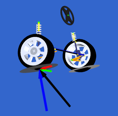
3D forces representation in the advanced model
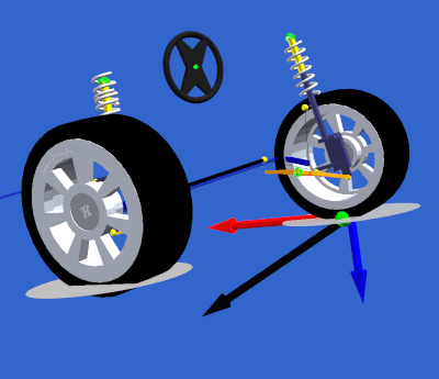
3D torques representation in the advanced model
REMARK:
For every force that you want to show, you will have to create a different vector, so a different .anim file. By default we allow the user to save up to 12 vectors, if you need more output value update the option
max_save_userwith the functionMbsDirdyn.set_options().
REMARK:
This feature is also valid for the analysis of inverse dynamics.