User constraints
The user constraints enable to impose constraints that can not be resolved using classical Robotran cuts.
The user constraint is expressed in the form: \(h_{usr}(q) = 0\)
The user has to provide, for a given configuration:
The value of the constraint: \(h_{usr}(q)\)
The Jacobian matrix of the constrain: \(J_{usr}(q)\)
The quadratic term: \(\left(\dot{J}\dot{q}(q, \dot{q})\right)_{usr}\)
The user constraints are implemented using the user_cons_hJ and user_cons_jdqd functions.
Back to the pendulum-spring example
The goal is to replace the prismatic joint between the pendulum and the slider by a screw joint. Since only simple joints can be implemented in Robotran, the screw joint will be modelled:
Using a rotoid and a prismatic joint along the same axis;
Adding a constraint to respect the screw thread:
Screw pitch : 20 mm.
The constraint can thus be written as: \(p\varphi - 2\pi z = 0\)
\(\varphi\): slider rotation along the pendulum;
\(z\): slider translation along the pendulum;
\(p\): the screw pitch
Step 1: Draw your multibody system
Open the Pendulum Spring model in MBsysPad:
Insert a R3 joint in the kinematic chain between the pendulum and the slider
See the tips and tricks if you don’t know how to modify the attach point of a body.
Give a name to the joint.
Set the R3 joint as dependent
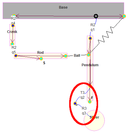
Illustration of the modified example with the screw joint
There is no specific action to do in MBsysPad for the user constraint.
Step 2: Generate your multibody equations
You have to generate the equations because we added a joint.
However if you add an user constraint on a existing project you don’t have to regenerate the equations because the user constraints are defined in the user functions.
Step 3: Write your user function
Edit the user_cons_hJ function:
Enter the expression of the constraint: \(h_{usr}(q)\)
Fill the jacobian matrix: \(J_{usr}(q)\)
import numpy as np

def user_cons_hJ(h, Jac, mbs_data, tsim):
   #...

   # define pitch value and retrieve joints ID
   p = 20e-3
   idT3 = mbs_data.joint_id["T3_slider"]
   idR3 = mbs_data.joint_id["R3_slider"]

   # define the value of the constraint
   h[1] = p*mbs_data.q[idR3]-2.*np.pi*mbs_data.q[idT3]

   # define the value of the jacobian matrix
   Jac[1,idR3] = p
   Jac[1,idT3] = -2*np.pi

   #...
Edit the user_cons_jdqd function:
No modification to do since the quadratic term of the constraint is null in the present case.
If the quadratic term of the constraint is nonzero you have to define it in this function.
Step 4: Run your simulation
Before running the simulation, you must modify the main script in order to indicate that there is a user constraint.
Open the main.py file and add mbs_data.set_nb_userc(1) after the
project loading and before the coordinate partitioning.
In addition, like for loop constraints, the script must call the coordinate partitioning before running the simulation. If it not already there, add the instructions to call the coordinate partitioning module:
Open the main.py file and add the following command
After the project loading (load() function)
Before the time integration (run() function)
#...

mbs_part = Robotran.MbsPart(mbs_data)
mbs_part.run()
# Run the coordinate partitioning process

#...
REMARK:
Some options are available for the coordinate partitioning process, see the documentation.
Check the results
The evolution of the system is the same as for the External forces part of the tutorial. This is due to the zero value of the inertia term of the Slider about the rotation axis. So the user constraint do not affect the dynamic of the rest of the system. Set a non-zero value and the rest of the system will be impacted.