User derivatives
It is possible to add additional constitutive equations to the equation of motion
This can be used to deal with multiphysics problem involving electrical circuits, pneumatics, hydraulics, …
The additional state equations will be added to the set of mechanical equations
In practice
The user must declare the state in a user model
The user must compute the state derivative equation in the user_Derivatives function
The state value can be accessed in any user function of the project
Back to the spring-pendulum example
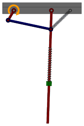
Pendulum spring illustration with torque
The exercise consists in adding an electrical DC motor to the pendulum example without the wall:
The motor will be connected to the revolute joint of the crank
The motor obeys the following relation
Electrical circuit equation: \(U_{mot} = R_{mot}*i_{mot}+k_{\phi}*\omega_{mot} + L \frac{di_{mot}}{dt}\)
Torque equation: \(T_{mot} = k_{\phi} * i_{mot}\)
A reductor is inserted between the motor and the axle: \(\begin{matrix} T_{axle} = \rho * T_{mot}\\ \omega_{axle} = \omega_{mot}/\rho \end{matrix}\)
The parameter values are:
\(U = 48\ V\)
\(k_{\phi} = 48.6\ mNm/A\)
\(\rho = 200\)
\(R_{mot} = 4.49\ \Omega\)
\(L = 0.573\ mH\)
Step 1: Draw your multibody system
Open the PendulumSpring model in MBsysPad
Add a user model for the motor
Add a scalar variable for each parameter
Add a state variable for the current
Set the nature of the :
crank joint to independent;
pendulum joint to dependent;
If you had modified the joint nature in the code in the previous section you have to update the code, modifications done in MBsysPad are overwritten.
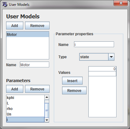
snapshot of the user model gui for introducing state variable
REMARK
Several state variables can be introduced either by introducing several values for a single state variable (state vector) or by defining several parameters with “state” type.
WARNING:
You can have two state variables with the same name in two different user model. However it is recommended to set an unique name for each state variable.
Step 3: Write your user function
Edit the user_Derivative function and introduce the state equation for the current:
def user_derivatives(mbs_data):
   #...

   id_crank = mbs_data.joint_id['R2_crank']
   rho = mbs_data.user_model['Motor']['rho']
   U   = mbs_data.user_model['Motor']['U']
   Rmot= mbs_data.user_model['Motor']['Rmot']
   kphi= mbs_data.user_model['Motor']['Kphi']
   L   = mbs_data.user_model['Motor']['L']

   # The user derivative index are retrieved in the user model state value.
   # This is important if your model contain more than one user state.
   id_state =  mbs_data.user_model['Motor']['i'][1]

   omMot = -mbs_data.qd[id_crank]*rho
   iMot = mbs_data.ux[id_state]
   mbs_data.uxd[id_state] = (U-Rmot*iMot-kphi*omMot)/L

   #...
REMARK
The user state vector is accessed via the ux field of the MbsData class
You can access to the ID of a state variable via the user model structure. If the state variable is a vector, you retrieve the ID of the first value of the vector in [1], second in [2], etc.
Edit the user_JointForces function and introduce the torque equation:
def user_JointForces(mbs_data,tsim):
   #...

   id_crank = mbs_data.joint_id['R2_crank']
   id_state =  mbs_data.user_model['Motor']['i'][1]

   iMot = mbs_data.ux[id_state]
   rho = mbs_data.user_model['Motor']['rho']
   kphi= mbs_data.user_model['Motor']['Kphi']

   mbs_data.Qq[id_crank] = -rho*kphi*iMot

   #...
   return
REMARK
The dynamics of the motor required a small time-step (smaller than the default one) or an adaptive integrator.
As result the simulation may be long. To reduce the simulation time you can multiply the motor inductance by a factor 10 without noticeable changes on the results
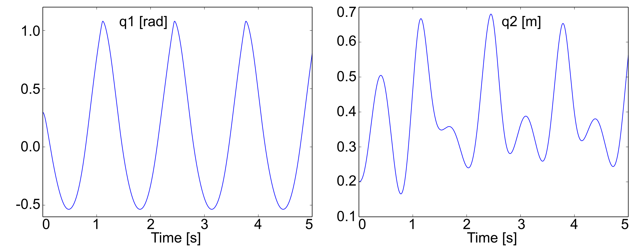
The time history of the motor current can be directly plotted from
the field ux of MbsDirdyn.results.
REMARK:
To let the motor rotate freely, the wall must be removed (by modifying the external forces).
REMARK:
The resolution of the motor dynamics requires a smaller time step than before. The computation time will increase.
You must edit the main function and decrease it :
mbs_dirdyn.set_options(dt0=1e-4)(except if you changed the inductance value).